8. Properties of Curves
a. Vector Functions, Position, Velocity and Plots
Not all vector functions are position vectors or parametric curves.
2. Vector Functions: Velocity and Force
Velocity
Three pages from now, we will define the velocity of a curve as the derivative of the position vector. \[ \vec{v}(t)=\langle v_1(t),v_2(t),v_3(t)\rangle =\dfrac{d\vec{r}}{dt} =\left\langle \dfrac{dx}{dt},\dfrac{dy}{dt},\dfrac{dz}{dt}\right\rangle \] We do not regard the velocity vectors as located at the origin. Rather, we regard the velocity vector \(\vec{v}(t)\) at time \(t\) to be located at the point \(\vec{r}(t)\), the tip of the position vector.
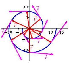
Plot the spiral \(\vec{r}(t)=(t\cos t,t\sin t)\), its position vector and its velocity vector \[ \vec{v}(t)=\langle \cos t-t\sin t,\sin t+t\cos t\rangle \] for \(\pi \le t \le 4\pi\). (You are not yet expected to be able to do all this yourself.)
The parametric curve is in blue.
Its position vector is in red.
Its velocity vector is in magenta.

Before defining the velocity, we need to define a derivative and before we define a derivative we need to define a limit.
Force
A force is an example of a vector field which we defined in the chapter on Vectors. To plot the force vector we put the tail of each vector at the point where it is evaluated. If an object moves along a curve due to the action of a force, then the force must be evaluated at the position of the particle, and we only plot the force vectors at points on the curve.
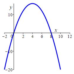
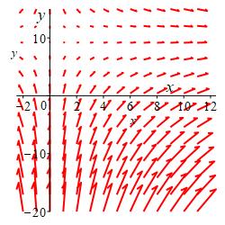
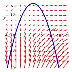
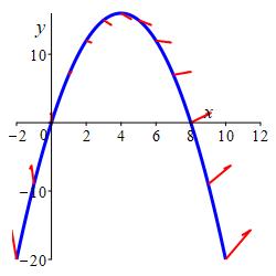
A charged particle moves along the parabola \(y=16-(x-4)^2\) parametrized as \(\vec{r}(t)=\left\langle t,16-(t-4)^2\right\rangle\) under the action of an electric field \(\vec{F}(x,y)=\left\langle x,10-y\right\rangle\) which on the curve is \(\vec{F}(t)=\left\langle t,(t-4)^2-6\right\rangle\). Plot the curve and the vector field for \(-2 \le t \le 10\).
The first two graphics show the curve and the electric field separately. The third graphic contains both the curve and the electric field superimposed in the same plot, and the last graphic shows the electric field expressed along the curve at integers from \(x=-2\) to \(x=10\). (Note: All the vectors have been shortened by a factor of \(8\) so the arrows will not overlap.)
Heading
Placeholder text: Lorem ipsum Lorem ipsum Lorem ipsum Lorem ipsum Lorem ipsum Lorem ipsum Lorem ipsum Lorem ipsum Lorem ipsum Lorem ipsum Lorem ipsum Lorem ipsum Lorem ipsum Lorem ipsum Lorem ipsum Lorem ipsum Lorem ipsum Lorem ipsum Lorem ipsum Lorem ipsum Lorem ipsum Lorem ipsum Lorem ipsum Lorem ipsum Lorem ipsum